The Drop
The Wi-Fi to the UGV drops out at 47 metres. It is not a clean disconnect. The link gets ratty for a few seconds, fades, comes back at 200 kbps for one suspicious frame, then disappears for good behind a concrete wall. The operator’s detection overlay freezes mid-scan. The autonomy hooks downstream of it stop receiving frames. Every piece of tooling that was watching the camera feed has nothing to watch.
This is the moment the project is built for. Wi-Fi remains the primary link in fair conditions. When it fails, an ESP-WIFI-MESH fallback delivers one usable still every five seconds, hopping through two mesh nodes between the vehicle and the operator, and the same downstream stack keeps working. Lower frame rate, same code path.
Two Orders of Magnitude
The fallback radio is not a video link. It cannot pretend to be one. ESP-WIFI-MESH gives roughly 0.5 Mbps usable across two hops, which is two orders of magnitude less than a healthy Wi-Fi connection.
One frame every five seconds is the design budget. Whatever passes through the radio has to fit, and the existing inference stack on the operator side has to consume it without modification. The interesting engineering happens at both ends of the link, not in the link itself.
UGV Side: 1,400× Smaller
A Raspberry Pi 4 handles capture. The camera produces a 3007×1991 frame at roughly 10 MB raw. Three steps reduce that to something a 0.5 Mbps link can deliver in time:
- Downscale to 640×480 with Lanczos resampling. The image goes from 10 MB to about 706 kB. Most of the gain is here, and it costs nothing the operator’s detection model cares about.
- mozjpeg at quality 5. Aggressive. Visibly artifacted. The output is 8.37 kB, with a follow-up lossless pass that saves another 16% on top.
- Base64 over UART to the ESP32. Roughly 33% of overhead, taking the on-wire size to about 11.16 kB.
An obvious question: why base64? Raw bytes would save 33% on the wire, and ESP-WIFI-MESH is a binary-clean transport. The constraint is one level lower. The serial console between the Pi and the ESP32 already carries telemetry, and the operator-side ESP32 prints into a stream the receiver script reads line by line. Sending raw binary into that stream collides with framing bytes and corrupts the telemetry path. Text encoding sidesteps the problem at the cost of a third more bytes per frame, which the radio can absorb at this cadence.
[info] target: 10240 bytes (10.0 kB)
[info] mozjpeg lossless saved 1644 bytes (16.1%)
[info] final:  640x480  q=5  8572 bytes (8.37 kB)
[info] base64: 11432 chars (11.16 kB on wire)
End-to-end, the camera-side pipeline shrinks the frame by roughly 1,400×. Most of that ratio comes from the resolution drop. The compression and encoding contribute the last factor of ten, and that last factor is what makes the link viable.
Two Hops, One Serial Line
The base64 string leaves the Pi over UART, gets handed to the ESP-WIFI-MESH stack, and traverses two intermediate mesh nodes before reaching the operator-side ESP32. Two hops adds latency and opportunities for retransmit, but it is what the deployment topology requires: the UGV is far enough out that direct line-of-sight to the operator is unreliable.
The receiver-side script reads the operator ESP32’s serial output, watches for the framing markers around an image payload, captures the bytes between them, and reassembles the base64. Telemetry lines outside the markers pass through to whatever is logging them. Two streams sharing one wire, demultiplexed at the destination.
Operator Side: FBCNN Restore
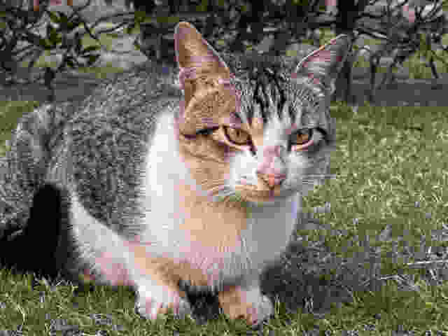
An 8 kB JPEG at quality 5 looks like an 8 kB JPEG at quality 5. There is heavy 8×8 blocking in flat regions, chroma bleeding around edges, and pink and magenta blotches in the white parts of the cat’s fur where the chroma subsampling collapsed. A YOLO model trained on natural images will still detect this, but the confidence drops and the bounding box can drift.
FBCNN (Flexible Blind CNN for JPEG artifact removal) is purpose-built for this exact failure mode. It takes the artifacted 640×480 in, predicts an internal quality embedding, and outputs a cleaned version at the same resolution.
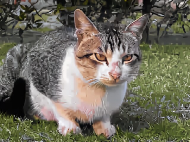
The original PyTorch model runs in roughly 22 seconds on the operator’s CPU per frame, which is too slow for a 5-second budget that already has upscale and inference downstream of it. Exporting to ONNX and running through ONNX Runtime drops that to about 9.8 seconds. The model is unchanged: same weights, same math. The runtime is what got better. ONNX Runtime fuses adjacent ops, pre-allocates buffers, and uses ARM and x86 SIMD kernels that PyTorch’s eager mode does not reach for at inference time.
[info] loading FBCNN ONNX...
[info] providers: ['CPUExecutionProvider']
[info] restoring 640x480_compressed.jpg...
[info] done in 9.8s; predicted QF: 92.2
[info] saved: 640x480_compressed_restored.png
One detail worth flagging. The model reports a predicted QF of 92.2 on an image the encoder produced at q=5. They are not the same number. FBCNN’s “QF” is an internal embedding that controls how aggressively the network cleans, not the literal libjpeg quality factor on the encoder side. Reading it as a literal QF will confuse you for an afternoon if you let it.
Operator Side: FSRCNN 4×
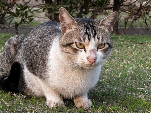
The detection model the operator runs on the Wi-Fi feed expects images at the camera’s native resolution, not 640×480. So the restored frame goes through a super-resolution step that produces a 2560×1920 output the downstream stack will accept without tensor-shape gymnastics.
FSRCNN is the choice here for one reason: speed. Newer architectures (Real-ESRGAN, SwinIR, EDSR) produce visibly sharper output, but on the operator’s CPU they cost between 30 seconds and several minutes per frame. FSRCNN finishes in about half a second, which preserves the per-frame budget. The result is softer than what a heavier model would produce, but the goal is to feed a detector, not to print the image at a gallery.
[info] input:  640x480
[info] scale:  4x FSRCNN
[info] output: 2560x1920
[info] done in 0.5s
[info] saved: 640x480_compressed_restored_4x_fsrcnn.png
Operator Side: Same YOLO
This is the slide that justifies the rest of the project.
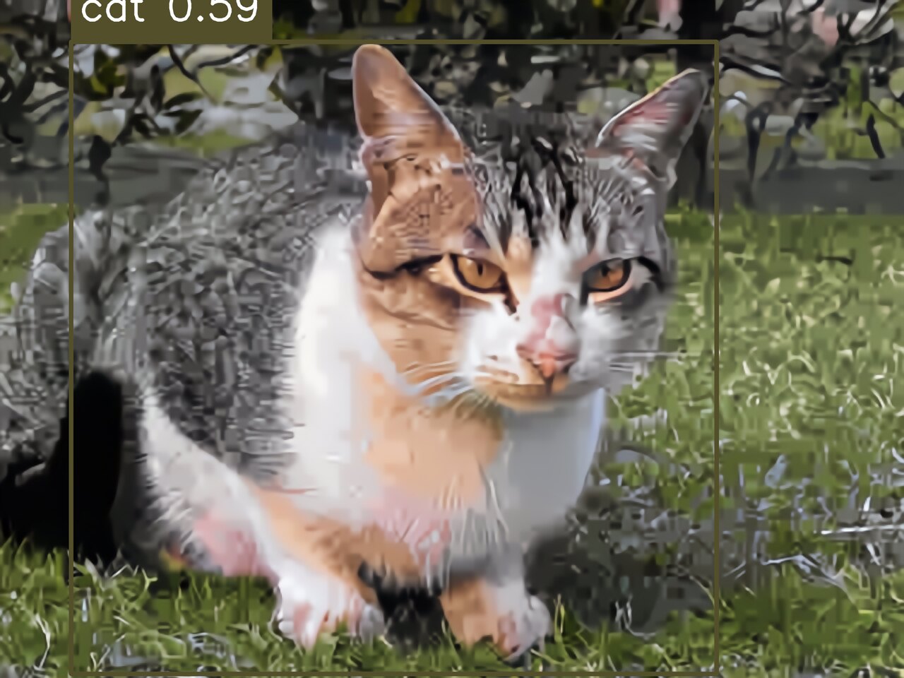
The 2560×1920 restored, upscaled image goes into the same YOLO inference pipeline that runs on the Wi-Fi feed. The detection script does not branch on which transport the image came from. It does not check the link state. It receives a tensor of the expected shape and runs the same call. The detection on this particular fallback frame: cat at confidence 0.59, bounding box from (201, 118) to (2029, 1908), in 0.72 seconds.
[info] running detection on 640x480_compressed_restored_4x_fsrcnn.png...
[info] detection done in 0.72s
  [cat] conf=0.59  box=(201,118)-(2029,1908)
[info] saved: 640x480_compressed_restored_4x_fsrcnn_detected.png
[info] 1 box(es) drawnConfidence is lower than what the operator sees on a clean Wi-Fi frame, where the same scene typically scores above 0.85. The drop reflects what was thrown away by the encoder and not fully recovered by FBCNN. For the existing autonomy hooks the detector feeds, 0.59 is well above their action threshold. The fallback is degraded, not broken.
The Numbers
The fallback path measured end-to-end, on production-equivalent hardware:
| Metric | Value | Notes |
|---|---|---|
| Bandwidth on the wire | ~11 kB / frame | base64 of an 8.4 kB JPEG |
| End-to-end latency | ~5 s | capture to operator screen |
| Effective throughput | ~0.2 fps | fallback cadence |
| Compression ratio | ~1,400× | raw camera frame to on-wire bytes |
| FBCNN inference | ~9.8 s | ONNX, CPU; was ~22 s in PyTorch |
| FSRCNN inference | ~0.5 s | CPU, 640×480 → 2560×1920 |
| YOLO detection | ~0.72 s | cat conf 0.59 on this frame |
| Mesh hops | 2 | UGV → node A → node B → operator |
The point of the project is not the compression ratio. It is the boundary that does not move when the radio does. Wi-Fi remains primary. When the link drops, the existing tooling, alerts, and autonomy hooks keep working through the fallback path at lower frame rate, and nothing downstream needs to know which radio delivered the frame.1
That is what graceful degradation looks like in the field. Not a banner that says “link lost.” A vision pipeline that quietly takes a hit on frame rate and keeps reporting.2
- A 1080×1080 carousel version of this writeup, intended for sharing, was generated alongside the post. The numbers in the carousel match the table above, with one rounded value in the bandwidth bar chart for legibility on mobile.
- There is one obvious next step: ship the same image both via Wi-Fi and via the mesh, run the inference twice, and have the consumer pick the higher-confidence result. The cost is a duplicated frame on a healthy link. The benefit is a system that is even less aware of which transport delivered the data. We have not built it yet.